We can ask if the conductance (7.1) computed using
transmission of left-side reservoir plane wave states through the QPC is equal
to that using right-side reservoir states.
Since the two directions correspond to opposite signs of ![]() ,
then in order to have linear response (well-defined
constant
,
then in order to have linear response (well-defined
constant ![]() around
around ![]() )
we would hope that they are equal.
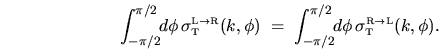
That the angular average of transmission cross section is equal
from the left and right sides is not immediately apparent in a general
asymmetric system.
For instance, consider Fig. 7.4b which has a small acceptance
angle from the left but a large from the right, therefore
very different forms of the
transmission cross sections
)
we would hope that they are equal.
That the angular average of transmission cross section is equal
from the left and right sides is not immediately apparent in a general
asymmetric system.
For instance, consider Fig. 7.4b which has a small acceptance
angle from the left but a large from the right, therefore
very different forms of the
transmission cross sections
![]() and
and
![]() .
.
If we assume classical motion then we can imagine a map from a Poincaré
Section (PS) ![]() at a vertical slice at
at a vertical slice at ![]() to another PS
to another PS
![]() at
at ![]() .
At each PS we consider only rightwards-moving (
.
At each PS we consider only rightwards-moving (![]() ) particles, and
take
) particles, and
take ![]() .
A certain area of phase space
.
A certain area of phase space ![]() is transmitted and is mapped
to an equal area in phase space
is transmitted and is mapped
to an equal area in phase space ![]() [88].
Time-reversal invariance holds since we consider magnetic field
[88].
Time-reversal invariance holds since we consider magnetic field ![]() ,
so we can negate the momenta (now considering
,
so we can negate the momenta (now considering ![]() ) and find that
the same phase space area is transmitted right-to-left.
When it is realised that the angle-averaged cross section is proportional
to the transmitted phase space area on a PS, then the symmetry
of the angle-averaged classical cross sections follows.
) and find that
the same phase space area is transmitted right-to-left.
When it is realised that the angle-averaged cross section is proportional
to the transmitted phase space area on a PS, then the symmetry
of the angle-averaged classical cross sections follows.
This is not obvious either for quantum cross sections, but it is also true.
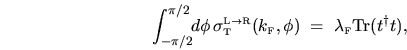
Comparing (7.11) with (7.14) gives
We now discuss a case in which non-thermal occupation
of incoming states is possible: the
rapidly developing field of coherent matter-wave optics, in which
potentials are defined by microfabricated structures
([76,191,16] and references therein).
There is a recent proposal [191] for observation of
quantization of atomic flux
through a micron-sized 3D QPC defined by the Zeeman effect potential of
a magnetic field.
The device is illuminated by a beam of atoms passing through a vacuum,
whose angular distribution is an experimental parameter
(for instance, a collimated oven source or a dropped cloud of cold atoms
[116]).
The atomic flux transmitted (per unit ![]() , at wavevector
, at wavevector ![]() ) will be
) will be
![]() where
where
![]() is the flux incident per unit wall area,
and we define the atomic `conductance' by
is the flux incident per unit wall area,
and we define the atomic `conductance' by
For an integer number of quantum channels, the
2D quantization of
![]() in units of
in units of ![]() [see Eq.(7.19]
becomes in 3D
the quantization of
[see Eq.(7.19]
becomes in 3D
the quantization of
![]() in units of
in units of ![]() [191,20,179].
As stated in Ref. [191], this accurate flux quantization
requires the incident beam width to be much larger than the QPC acceptance
angle.
[191,20,179].
As stated in Ref. [191], this accurate flux quantization
requires the incident beam width to be much larger than the QPC acceptance
angle.
Eq.(7.25) is the matter-wave equivalent of Eq.(7.11), with the important difference that it has a general weight function. Non-uniformity of this weight function leads to a key result: that asymmetry of the conductance is possible given identical illumination on either side, even though the (center of mass) motion is time-reversal invariant. For example, if the incident flux used to illuminate the horn QPC of Fig. 7.4b is narrow in angular spread, then the left-to-right conductance will be much larger than the right-to-left conductance. This contrasts with the 2DEG case where the conductance is always symmetric.
Finally, it is interesting to note that for the non-thermal
incident (reservoir) distributions
discussed above, the
Landauer formula has the modified form