Computational Lab #3: introduction to iterative methods

Math 56, Winter 2025

See the course GitHub page to download the notebook. Make sure to respond to all questions!

import numpy as np
import matplotlib.pyplot as plt

from lab3_helper_funcs import *

Problem 1

In this question, you will compare Richardson’s method (gradient descent with fixed stepsize) with steepest descent (with variable stepsize).

n = 200
np.random.seed(0)
A = np.random.normal(size=n)
A = (A.T @ A) + 1e-1*np.eye(n)
xtrue = np.random.normal(size=n)
b = A @ xtrue

Part (a): Complete the following functions for Richardson’s method and steepest descent.

def richardson(A, b, n_iterations=25, alpha=1.0, x0=None):
    
    # Initialization if none given
    if x0 is None:
        x = np.zeros(len(b))
    else:
        x = x0.copy()


    r = b - A @ x
    residual_norms = [ np.linalg.norm(r) ]
    solution_history = [ x.copy() ] 
    for j in range(n_iterations):
        
        ## Your code here


        residual_norms.append( np.linalg.norm(r) )
        solution_history.append(x.copy())

    return x, residual_norms, solution_history

def steepest_descent(A, b, n_iterations=25, x0=None):

    # Initialization if none given
    if x0 is None:
        x = np.zeros(len(b))
    else:
        x = x0.copy()

    r = b - A @ x
    residual_norms = [ np.linalg.norm(r) ]
    solution_history = [ x.copy() ] 
    for j in range(n_iterations):
        
        # Your code here

        residual_norms.append( np.linalg.norm(r) )
        solution_history.append(x.copy())

    return x, residual_norms, solution_history

    

Part (b): Make a plot (or two) that verifies that Richardson’s method converges when the stepsize parameter satisfies \(\alpha < \frac{2}{\lambda_{\text{max}}(\mathbf{A})}\).

Part (c): Compare the performance of steepest descent with Richardson’s method (using a good stepsize). What do you observe?

Problem 2

Next, we will compare steepest descent with the conjugate gradient method.

A = np.load("q2_A.npy")
n = A.shape[0]
xtrue = np.ones(n)
b = A @ xtrue

Part (a): Complete the following function for the conjugate gradient (CG) method.

def conjugate_gradients(A, b, n_iterations=25, x0=None):

    # Initialization if none given
    if x0 is None:
        x = np.zeros(len(b))
    else:
        x = x0.copy()

    r = b - A @ x # set r0
    d = r # set d0 = r0

    residual_norms = [ np.linalg.norm(r) ]
    solution_history = [ x.copy() ] 
    for j in range(n_iterations):

        # Your code here
        

        residual_norms.append( np.linalg.norm(r) )
        solution_history.append(x.copy())

    return x, residual_norms, solution_history

    

Part (b): Make a plot using plt.semilogy() which verifies the error bound \[ \| \mathbf{x}^* - \mathbf{x}_k \|_{\mathbf{A}} \leq \left( \frac{ \kappa - 1 }{ \kappa + 1 } \right)^k \| \mathbf{x}^* - \mathbf{x}_0 \|_{\mathbf{A}} \] for steepest descent, as well as the error bound \[ \| \mathbf{x}^* - \mathbf{x}_k \|_{\mathbf{A}} \leq 2 \left( \frac{ \sqrt{\kappa} - 1 }{ \sqrt{\kappa} + 1 } \right)^k \| \mathbf{x}^* - \mathbf{x}_0 \|_{\mathbf{A}} \] for the CG method. Describe anything that you notice about the behavior of the curves.

Response:

Part (c): Based on our discussions in class, can you explain why the CG method converges so quickly for this matrix \(\mathbf{A}\)?

Problem 3

In this problem, you will investigate the preconditioned conjugate gradient method. Load the matrices \(\mathbf{L}\) and \(\mathbf{W}\), and then form the matrix \(\mathbf{A} = \mathbf{L}^T \mathbf{W} \mathbf{L}\).

L = np.load("q3_L.npy")
W = np.load("q3_W.npy")
A = L.T @ W @ L

plt.imshow(L)
plt.show()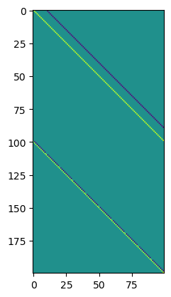

Part (a): Draw a random vector \(\mathbf{b}\) and solve \(\mathbf{A} \mathbf{x} = \mathbf{b}\) using CG. Then, solve the same system but using preconditioned CG with preconditioner \(\mathbf{M} = \mathbf{L}^T \mathbf{L}\). Make a plot of the iteration index versus the residual norm.

np.random.seed(0)
M = L.T @ L
b = np.random.normal(size=A.shape[0])

def preconditioned_conjugate_gradients(A, b, M, n_iterations=25, x0=None):

    if x0 is None:
        x = np.zeros(len(b))
    else:
        x = x0.copy()

    r = b - A @ x  # Initial residual r0
    z = np.linalg.solve(M, r)  # Preconditioned residual z0
    d = z.copy()  # Initial direction

    residual_norms = [np.linalg.norm(r)]
    solution_history = [x.copy()]

    for j in range(n_iterations):
        Ad = A @ d
        alpha = np.dot(r, z) / np.dot(d, Ad)  # Step size
        x += alpha * d  # Update solution
        r_new = r - alpha * Ad  # Update residual
        z_new = np.linalg.solve(M, r_new)  # Apply preconditioner
        beta = np.dot(r_new, z_new) / np.dot(r, z)  # Update coefficient
        d = z_new + beta * d  # Update direction

        r, z = r_new, z_new  # Update residuals for next iteration
        residual_norms.append(np.linalg.norm(r))
        solution_history.append(x.copy())


    return x, residual_norms, solution_history

Part (b): Can you explain why \(\mathbf{M}\) is a good preconditioner? Make a plot to support your answer.

Response:

Bonus: modify your code for preconditioned CG so that any factorization of \(\mathbf{M}\) used for applying \(\mathbf{M}^{-1}\) is re-used across the iterations of preconditioned CG.