
Math 76
Introduction to Bayesian Computation
Question 1
Micro x-ray computed tomography ($\mu$-CT) is a technique used to image the internal three dimensional structure of objects. CRREL has a $\mu$-CT scanner that is commonly used to study water content in snow and sand. Below is a single two dimensional slice of moist sand taken with the CRREL $\mu$-CT scanner. There are three obvious phases in the image: pore space (black), sand grains (dark gray), and water (light gray). Each pixel has a certain intensity in the set $[0,256]\subseteq\mathbb{R}$. The bright pixels have a high intensity, the dark pixels have a low intensity.
Given a $\mu$-CT image, we are often interested in classifying each of the pixels as being either pore space, sand grains, or water. This question considers that classification problem probabilistically.
Let $C_j$ denote the class of pixel $j$ (either grain, pore, or water). Assume $65\%$ of the pixels are grain, $25\%$ are pores, and $10\%$ are water. Let $I_j$ denote the intensity of pixel $j$. Assume that the intensity of grain pixels follows a Gaussian distribution with mean $\mu_g=200$ and variance $\sigma_g^2=100$, the intensity of pore pixels follows a Gaussian distribution with mean $\mu_p=25$ and variance $\sigma_p^2 = 100$, and the intensity of water pixels follows a Gaussian distribution with mean $\mu_w=150$ and variance $\sigma_w^2 = 1600$.
- What are the sample spaces of $C_j$ and $I_j$?
- Assume you observe an intensity of $\hat{I}$ for pixel $j$. Use Bayes’ rule to derive expressions for the probability that this pixel is in each class given the observation $I_j=\hat{I}$. Make sure to justify any assumptions you make.
- Use your expression from part (b) to compute the probability of a pixel being in each class when the pixel was observed to have an intensity of $\hat{I}=20$. Then try $\hat{I}=140$. Explain your findings intuitively based on the means and variances for each class.
Part 1 Solution
The sample space of the class random variable $C_j$, denote here by $\Omega_C$, describes the different possible classes, which are $\Omega_C = {Grain, Pore, Water}$. To simplify the notation below, we will just use the first letter of each class name, which results in in $\Omega_C = {G,P,W}$.
We are representing the intensities of each class as Gaussian distributions. This implies that the samples space of the intensity is the same as the support of a Gaussian density, which is $\Omega_I=(-\infty,\infty)$. However, the actual values returned by the $\mu$-CT are in $\Omega_I=[0,256]$. Either option will be accepted.
Part 2 Solution
From the problem description, we know that the intensity within each class follows a Gaussian distribution \(\begin{eqnarray} f(I_j | C_j=G) &=& N(\mu_g, \sigma_g^2)\\ f(I_j | C_j=P) &=& N(\mu_p, \sigma_p^2)\\ f(I_j | C_j=W) &=& N(\mu_w, \sigma_w^2). \end{eqnarray}\) The fraction of the pixels in each class can be used to construct prior probabilities that a single pixel is in a particular class, i.e., \(\begin{eqnarray} \mathbb{P}[C_j=G] &=& 0.65\\ \mathbb{P}[C_j=P] &=& 0.25\\ \mathbb{P}[C_j=W] &=& 0.1. \end{eqnarray}\)
We are interested in the probability of being in each class given the observed intensity $\hat{I}$, e.g., $\mathbb{P}[C_j=G | \hat{I}]$. While we don’t know this probability directly, Bayes’ rule provides a way of computing such posterior probabilities in terms of the intensity distrbution for each class and the overall fraction of each class. For each class $k$, Bayes’ rule gives \(\mathbb{P}[C_j=k | I_j = \hat{I}] = \frac{f(\hat{I} | C_j=k) \mathbb{P}[C_j=k]}{f(\hat{I} | C_j=G) \mathbb{P}[C_j=G] + f(\hat{I} | C_j=P) \mathbb{P}[C_j=P]+ f(\hat{I} | C_j=W) \mathbb{P}[C_j=W]}\)
Part 3 Solution
While code is not required for solving this problem, here we use some python code to compute the posterior probabilities for each class. It is perfectly fine to do all of these calculations by hand as well.
from scipy.stats import norm
import numpy as np

num_classes = 3
likely_means  = np.array([200, 25, 150]) # The means of the the Gaussian likelihoods
likely_vars = np.array([100, 100, 1600]) # The variances of the Gaussian likelihoods
prior_probs = np.array([0.65, 0.25, 0.1]) # Prior probabilites for each class

def PostProbs(Ihat):
    """ Computes the posterior probabilities of being in each class
        given an observed intensity Ihat.
    """
    likelies = norm.pdf(Ihat, loc=likely_means, scale=np.sqrt(likely_vars))
    evidence = np.sum(likelies*prior_probs)
    return likelies*prior_probs / evidence

Ihat = 20
probs20 = PostProbs(Ihat)

Ihat = 140
probs140 = PostProbs(Ihat)
The resulting posterior probabilities for $\hat{I}=20$ are
| Class | $\mathbb{P}[C_j=k \mid \hat{I}=20]$ |
|---|---|
| Grain | 0.00 |
| Pore | 1.00 |
| Water | 0.00 |
and for $\hat{i}=140$,
| Class | $\mathbb{P}[C_j=k \mid \hat{I}=20]$ |
|---|---|
| Grain | 0.00 |
| Pore | 0.00 |
| Water | 1.00 |
Of course, the probability of being in each these classes is not exactly $1$, but slightly less than one. Regardless, the results make intuitive sense because the posterior probabilities are largest for the class with a mean intensity that is closest to the observed intensity. The fact that the posterior probability collapses onto a single class is a result of the likelihood functions for the grain and pore classes having relatively small variances. This results in little overlap of the Gaussian likelihood functions for those two classes.
Question 2
In class we have often used the “unknown mean known variance” Gaussian model. In that setting, the likelihood function resembled a Gaussian PDF with our parameter of interest playing the role of the mean. An alternative, that we consider in this question, is the “known mean unknown variance” Gaussian model, where the likelihood function still resembles a Gaussian PDF but where the variance of the Gaussian is the parameter of interest.
Assume $Y\sim N(0,\sigma^2)$ is a zero mean normal random variable and let $y_1, y_2, \ldots, y_N$ denote $N$ observations of $Y$. Here we assume that $\sigma^2$ is unknown and needs to be characterized from the observations $y_1, \ldots, y_N$. We will assume a inverse-Gamma prior on $\sigma^2$, which has a density of the form \(f(\sigma^2) = \frac{\beta^\alpha}{\Gamma(\alpha)} (\sigma^{2})^{-\alpha-1} e^{-\frac{\beta}{\sigma^2}}\) for some parameters $\alpha$ and $\beta$.
- What is the likelihood function $f(y \mid \sigma^2)$ for a single observation of $Y$.
- Show that the inverse-Gamma density above is a conjugate prior for the likelihood function from part 1. Use $\alpha_1$ and $\beta_1$ to denote the posterior parameters. Normalizing constants can be ignored or simply expressed as constants in your work.
- Write out Bayes’ rule for the situation where $N$ observations are available and use the result from part 2 to find an expression for the posterior parameters $\alpha_N$ and $\beta_N$ after $N$ observations. Make sure to show your work and describe any assumptions you might make to help simplify the problem.
Part 1 Solution
The likelihood function stems from the distribution of the random variable $Y$, which has zero mean and unknown variance $\sigma^2$. For a single observation $y$, the likelihood function therefore takes the form \(\begin{eqnarray} f(y|\sigma^2) &=& \frac{1}{\sqrt{2\pi\sigma^2}}\exp\left(-\frac{y^2}{2\sigma^2}\right)\\ &=& \frac{1}{\sqrt{2\pi}}(\sigma^2)^{-1/2}\exp\left(-\frac{y^2}{2\sigma^2}\right) \end{eqnarray}\) Notice that the variance $\sigma^2$ appears in both the normalizing constant and in the exponential.
Part 2 Solution
Using Bayes’ rule, we can write the posterior density as \(f(\sigma^2 | y) = C f(y|\sigma^2) f(\sigma^2),\) where $1/C = \int f(y|\sigma^2) f(\sigma^2) d\sigma^2$ is the evidence, which does not depend on the value of $\sigma^2$. Plugging in the forms of the likelihood and prior, we have
\(\begin{eqnarray} f(\sigma^2 | y) &=& = C f(y|\sigma^2) f(\sigma^2)\\ &=& C \frac{1}{\sqrt{2\pi}}(\sigma^2)^{-1/2}\exp\left(-\frac{y^2}{2\sigma^2}\right) \frac{\beta^\alpha}{\Gamma(\alpha)} (\sigma^{2})^{-\alpha-1} \exp\left[-\frac{\beta}{\sigma^2}\right]\\ &=&\frac{C \beta^\alpha}{\sqrt{2\pi}\Gamma(\alpha)}(\sigma^2)^{-1/2}\exp\left(-\frac{y^2}{2\sigma^2}\right) (\sigma^{2})^{-\alpha-1} \exp\left[-\frac{\beta}{\sigma^2}\right]\\ &=&\frac{C \beta^\alpha}{\sqrt{2\pi}\Gamma(\alpha)}(\sigma^2)^{-\alpha-3/2}\exp\left(-\frac{1}{\sigma^2}\left(\frac{y^2}{2}+\beta\right)\right)\\ &=&C_1(\sigma^2)^{-\alpha-3/2}\exp\left(-\frac{1}{\sigma^2}\left(\frac{y^2}{2}+\beta\right)\right)\\ \end{eqnarray}\) Matching the $\sigma^2$ terms in this expression with the $\sigma^2$ terms in the inverse-Gamma density, we see that this expression is also an inverse-Gamma density with parameters $\alpha_1$ and $\beta_1$ defined by \(\begin{eqnarray} \alpha_1 &=& \alpha + \frac{1}{2}\\ \beta_1 &=& \beta + \frac{y^2}{2}\\ \end{eqnarray}\)
Part 3 Solution
Now consider the case where we have $N$ observations $y_1,\ldots, y_N$. Bayes’ rule is then given by \(f(\sigma^2 \mid y_1, \ldots, y_N) \propto f(y_1, \ldots, y_N \mid \sigma^2) f(\sigma^2).\) Assuming the observations are conditionally independent given $\sigma^2$, we can simplify the likelihood function to obtain \(\begin{eqnarray} f(\sigma^2 \mid y_1, \ldots, y_N) &\propto& f(\sigma^2)\prod_{i=1}^N f(y_i \mid \sigma^2)\\ &\propto& f(y_N \mid \sigma^2) f(\sigma^2)\prod_{i=1}^{N-1} f(y_i \mid \sigma^2). \end{eqnarray}\) The second line of this expression indicates a recursive form form Bayes’ rule that is more convenient for deriving the posterior parameters $\alpha_N$ and $\beta_N$. In particular, notice that \(f(\sigma^2 \mid y_1,\ldots, y_{N-1})\propto f(\sigma^2)\prod_{i=1}^{N-1} f(y_i \mid \sigma^2),\) which implies the recursion \(f(\sigma^2 \mid y_1, \ldots, y_N) \propto f(y_N | \sigma^2) f(\sigma^2 | y_1, \ldots, y_{N-1}).\) Thus, the posterior density $f(\sigma^2 \mid y_1,\ldots,y_{N-1})$ after $N-1$ steps is “updated” to created the posterior after $N$ steps by multiplying by the Gaussian likelihood function $f(y_N\mid\sigma^2)$. From parts 1 and 2 of this question we know that if the posterior after $N-1$ observations follows an inverse-Gamma density, then the posterior after $N$ observations will also be inverse-Gamma with parameters given by \(\begin{eqnarray} \alpha_N &=& \alpha_{N-1} + \frac{1}{2}\\ \beta_N &=& \beta_{N-1} + \frac{y_N^2}{2}. \end{eqnarray}\) Applying this recursion for all $N$ steps, yields an expression for the posterior parameters $\alpha_N,\beta_N$ in terms of the prior parameters $\alpha,\beta$ and the observations: \(\begin{eqnarray} \alpha_N &=& \alpha + \frac{N}{2}\\ \beta_N &=& \beta + \frac{1}{2}\sum_{i=1}^Ny_i^2. \end{eqnarray}\)
Question 3
Suppose we are interested in the outcome of a political election with two candidates $C_1$ and $C_2$ who are in political parties $P_1$ and $P_2$, respectively. Candidates from party $P_1$ have won 7 out of the last 10 elections. In a poll of $100$ people however, candidate $C_2$ was preferred by $60$ people while candidate $C_1$ was preferred by the remaining $40$ people. The question is, what is the probability that candidate $C_1$ will win the election?
This is a modeling question and therefore has more than one right answer. To get full credit, you must describe your approach in detail and clearly identify any assumptions you make. Grading criteria is provided in the table below to help guide your solution. Note the requirement to use a Beta prior density somewhere in your analysis.
Grading Criteria:
| Requirement | |
|---|---|
| Was a Beta prior density used anywhere in the analysis? | Yes/No |
| Were all assumptions clearly listed? | Yes/Partially/No |
| Are the assumptions valid? | Yes/Somewhat/No |
| Were the previous election results used in the analysis? | Yes/No |
| Were the polling results used in the analysis? | Yes/No |
| Were there any mathematical errors? | Yes/No |
One Possible Solution
To assess the probability that $C_1$ will win, we will first consider another random variable $X$ representing the vote of a person in the electorate. We assume that there are no third party candidates and thus the sample space of $X$ is $\Omega_x={C_1,C_2}$, implying that $X$ is thus a Bernoulli random variable with some unknown parameter $p$ representing the probability that someone will vote for candidate $C_1$. Our goal is to construct a probability distribution over the parameter $p$ that acccounts for the given historical election and recent poll results.
Assume there are $M$ voters in the electorate and that the same number of voters participated in previous elections. Also assume that each vote is independent (given the value of $p$), which allows us to represent the total number of votes for candidate $C_1$ as a Binomial random variable with the same probability $p$. Let $M_1$ denote this Binomial random variable.
Now assume that the candidate who gets the most votes wins (e.g., ignore anything like the electoral college). The probability that $M_1$ garners the majority of the votes, and therefore wins, can be mathematically expressed as
\(\begin{eqnarray} \mathbb{P}\left[ M_1 > \frac{M}{2} \right] &=& \int_0^1 \mathbb{P}\left[ \left. M_1 > \frac{M}{2} \right| p\right] f(p) dp\\ & = & \int_0^1 \left[1-F\left(\left.\frac{M}{2} \right| p\right)\right] f(p) dp\\ & = & 1- \int_0^1 F\left(\left.\frac{M}{2} \right| p\right)f(p) dp\\ \end{eqnarray}\) where $F(\cdot|p)$ denotes the binomial CDF of the votes for $M_1$ given the value of $p$ and $f(p)$ denotes the probability density function over $p$.
For a large electorate $M$, the binomial CDF $F(M/2 \mid p)$ can be well approximated by an indicator function $I[p\geq 0.5]$. If $p>0.5$, then as $M\rightarrow \infty$, $\mathbb{P}[M_1\geq M/2] \rightarrow 1$ and $\mathbb{P}[M_1<M/2]\rightarrow 0$. Thus, we can approximate the probability of candidate $C_1$ winning by the probability that the parameter $p$ is greater than $0.5$:
\[\begin{eqnarray} \mathbb{P}\left[ M_1 > \frac{M}{2} \right] & \approx & \int_0^1 I\left[ p \geq 0.5 \right] f(p) dp\\ &=& \mathbb{P}[p \geq 0.5] \end{eqnarray}\]Prior Distribution
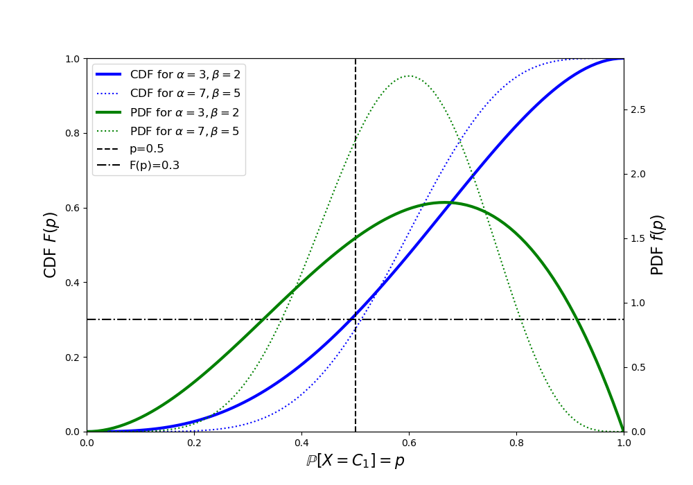
Party $P_1$ has won $7$ out of the last $10$ elections. This seems to imply that the probability of party $P1$ winning an election is about $0.7$. Notice however, that there is not a direct link between the probability that the party wins and the probability that a voter will vote for the candidate from party $P_1$. If the electorate has not changed and everyone who voted for party $P1$ in the previous election votes for candidate $C1$ in the current election, then the historical results only tell us that the probability that more than half the electorate will vote for $C1$ is approximately $0.7$. Using the approximation to the success probability describe above, this implies
\[\begin{eqnarray} \mathbb{P}[p\geq0.5]\approx 0.7\\ \Rightarrow \mathbb{P}[p<0.5]\approx 0.3 \end{eqnarray}\]The beta distribution is often used to model random variables, like the Bernoulli probability $p$, with sample spaces over $[0,1]$. We will therefore employ a beta prior distribution and try to find parameters $\alpha$ and $\beta$ that respect the previous election results without overly constraining the values of $p$. A prior distribution that is concentrated near a single value of $p$ would not allow for the potentially significant differences between voter preferences for candidate $C_11$ and voter preferences for previous candidates for party $P_1$.
As shown in the plot below, values of $\alpha=3$ and $\beta=2$ respect the historical election results (i.e., $\mathbb{P}[p<0.5]\approx 0.3$) while still having a non-negligible density over most of the parameter space. Notice that values of $\alpha=7$ and $\beta=5$ which could be motivated by simply counting the number of success and failures of party $P1$ in the past also respect the previous election results, but put more confidence in the value of $p$.
Likelihood Function
To define a relationship between $p$, which denotes the probability someone will vote for $C_1$ in the election, we assume that voter preferences do not change over time, so the poll results show exactly how the $100$ people polled will vote in the election. Like the votes themselves, we also assume that the poll responses are independent given the parameter $p$. Under these assumptions, we can use a binomial likelihood function to relate $p$ to the 40 “successes” and 60 “failures” in the poll. Note that this implicitly ignores any systematic bias that might exist in the peopled polled are representative of the general electorate.
Posterior Probabilities We know from class that a beta prior is conjugate to a binomial likelihood, which means that the posterior will also be from the beta family of distributions. Let $\alpha$ and $\beta$ denote the parameters of the prior beta distribution and let $\alpha^\ast$ and $\beta^\ast$ denote the parameters of the posterior beta distribution. We know that for $40$ successes and $60$ failures in the binomial likelihood, the posterior parameters are given by
\[\begin{eqnarray} \alpha^\ast &=& \alpha + 40 = 43\\ \beta^\ast &=& \beta + 60 = 62 \end{eqnarray}\]The posterior density using these values is plotted below.
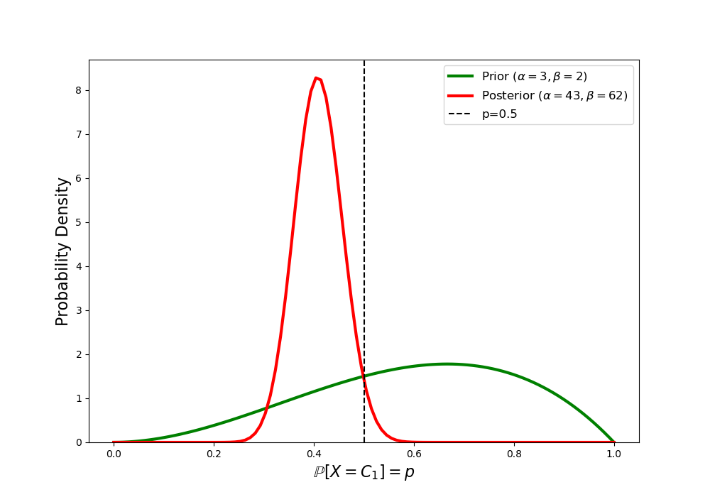
The probability that candidate $C_1$ will get more votes than candidate $C_2$ can then be approximated as the probability that $p$ is greater than $0.5$ (recall the discussion above on this point). Using SciPy Stats to evaluate the CDF of the beta distribution, we have
\[\boxed{ \begin{eqnarray} \mathbb{P}[C_1\text{ wins}]&\approx& \mathbb{P}[p\geq0.5]\\ &=& 1-0.97\\ &=&0.03. \end{eqnarray} }\]Question 4
Imagine someone who develops a fever in New England during the summer. They may have either COVID-19 ( C ), Lyme Disease (L), or the flu (F). From historical data, we might estimate that $\mathbb{P}[C] = 0.1$, $\mathbb{P}[L] = 0.5$, $\mathbb{P}[F]=0.4$. Given the current pandemic, this person receives a COVID-19 test. We denote the event of a positive test by P and the event of a negative test by $N$. Assume a false negative rate of $\mathbb{P}[N \mid C] = 0.05$ and false positive rates of $\mathbb{P}[P \mid L] = 0.02$ and $\mathbb{P}[P \mid F] = 0.03$.
- What is the marginal probability of a positive test result $c$?
- What is the joint probability that this person has Lyme disease and a positive test $\mathbb{P}[L,P]$?
- What is the probability that this person has the flu given a negative COVID-19 test $\mathbb{P}(F \mid N)$ ?
Part 1 Solution
\(\begin{eqnarray} \mathbb{P}[P] &=& \mathbb{P}[P|C]\mathbb{P}[C] + \mathbb{P}[P|L]\mathbb{P}[L] + \mathbb{P}[P|F]\mathbb{P}[F]\\ &=& (0.95)(0.1) + (0.02)(0.5) + (0.03)(0.4)\\ &\approx& 0.12 \end{eqnarray}\)
Part 2 Solution
\(\begin{eqnarray} \mathbb{P}[L,P] &=& \mathbb{P}[P|L]\mathbb{P}[L]\\ &=& (0.02)(0.5)\\ & = & 0.01 \end{eqnarray}\)
Part 3 Solution
\(\begin{eqnarray} \mathbb{P}[F | N] &=& \frac{\mathbb{P}[N|F] \mathbb{P}[F]}{\mathbb{P}[N]}\\ &=& \frac{\mathbb{P}[N|F] \mathbb{P}[F]}{1-\mathbb{P}[P]}\\ &=& \frac{(0.97)(0.4)}{1 - 0.12}\\ &\approx& 0.44 \end{eqnarray}\)
Question 5
- The information entropy of a continuous random variable $X$ with probability density function $f(x)$ is given by $\mathbb{E}[-\log(f(x))]$. What is the information entropy of a random variable with sample space $\Omega_x=[1,2]$ and density $f(x) = \frac{2}{3}x$?
- Consider a random variable $X$ with sample space $[-1,1]$ and probability density function $f(x) = \frac{3}{2} x^2$. What is the variance of $X$?
- Consider a Roulette wheel at a Las Vegas casino. When spun, a ball will randomly drop into one of 38 possible slots. Two of the slots are green (0 and 00), 18 of the slots are black and 18 of the slots are red. The ball is equally likely to fall into each slot. When someone bets \$1 on black, they will get their money back and receive an additional \$1 if the ball lands on black. However, they will lose their bet if the balls lands on red or green. What is the expected return on a \$1 bet? Will the casino make money on average?
Part 1 Solution
\(\begin{eqnarray} \mathbb{E}[-\log(f(x))] & = & -\int_{\Omega_x} \log(f(x)) f(x) dx\\ & = & -\frac{2}{3} \int_{1}^2 \log\left(\frac{2}{3}x\right) x dx\\ & = & -\frac{2}{3} \int_{1}^2 \log\left(\frac{2}{3}\right)x + \log(x) x dx\\ & = & -\frac{2}{3}\log\left(\frac{2}{3}\right) \left( \frac{1}{2}x^2 \right)_1^2 - \frac{2}{3} \int_1^2 x \log(x) dx\\ & = & -\frac{2}{3}\log\left(\frac{2}{3}\right) \frac{3}{2} - \frac{2}{3} \int_1^2 x \log(x) dx\\ & = & -\log\left(\frac{2}{3}\right)- \frac{2}{3}\left[ \frac{1}{2}x^2\log(x) - \frac{1}{4}x^2\right]_1^2 \\ & = & -\log\left(\frac{2}{3}\right) - \frac{2}{3}\left[ 2\log(2) - 1 + \frac{1}{4}\right]\\ &\approx& -0.019 \end{eqnarray}\)
Part 2 Solution
Before computing the variance, we need to compute the mean: \(\begin{eqnarray} \mathbb{E}[X] &=& \int_{-1}^1 x f(x) dx\\ &=& \int_{-1}^1 x \frac{3}{2}x^2 dx\\ & = & \left.\frac{3}{8} x^4 \right|_{-1}^1\\ & =& 0 \end{eqnarray}\) The variance is then given by \(\begin{eqnarray} \text{Var}[X] &=& \mathbb{E}[(X-\mathbb{E}[X])^2]\\ &=& \mathbb{E}[X^2]\\ & = & \int_{-1}^1 x^2 \frac{3}{2}x^2 dx\\ &=& \left. \frac{3}{10} x^5 \right|_{-1}^1\\ &=& 0.6 \end{eqnarray}\)
Part 3 Solution
Here we consider the expected return on a \$1 bet on black. The return is \$2 if the ball lands on black and \$0 otherwise. This can be described mathematically as $2 I(X=B)$, where $I(X=B)$ is an indicator function that the random variable $X$ lands on black. \(\begin{eqnarray} \mathbb{E}\left[ 2 I(X=B) \right] & = & 2\mathbb{P}[B]\\ & = & 2 \frac{18}{38}\\ & \approx & 0.95 \end{eqnarray}\) Thus, the expected return on a \$1.00 bet is \$0.95. No surprisingly, The gambler is losing money on average and the casino is earning money on average.