LAR Singular Value Decomposition

Section 3.6 Singular Value Decomposition

We show how the spectral decomposition for Hermitian matrices gives rise to an analogous, but very special decomposition for an arbitrary matrix, called the singular value decomposition (SVD).

We shall state without proof the version of the SVD which holds for linear transformations between finite-dimensional inner product spaces, but its statement is so elegant, it’s depth of importance is almost lost.

Then we state and prove the matrix version, providing some examples to demonstrate its utility.

Subsection 3.6.1 SVD for linear maps

We begin with a statement of the singular value decomposition for linear maps as paraphrased from Theorem 6.26 of [1].

Theorem 3.6.1.

Let \(V,W\) be finite-dimensional inner product spaces and \(T:V\to W\) a linear map having rank \(r.\) Then there exist orthonormal bases \(\{v_1, \dots, v_n\}\) for \(V\) and \(\{w_1, \dots, w_m\}\) for \(W,\) and positive scalars \(\sigma_1\ge \dots \ge \sigma_r\) so that

\begin{equation*} T(v_i) = \begin{cases} \sigma_iu_i\amp \text{ if }1 \le i \le r\\0\amp \text{ if }i \gt r.\end{cases} \end{equation*}

Moreover, the \(\sigma_i\) are uniquely determined by \(T,\) and are called the singular values of \(T.\)

Another way to state the main part of this result is the if the orthonormal bases are \(\cB_V=\{v_1, \dots, v_n\}\) and \(\cB_W = \{w_1, \dots, w_m\}\text{,}\) then the matrix of \(T\) with respect to these bases has the form

\begin{equation*} [T]_{\cB_V}^{\cB_W} = \ba{rr}D\amp 0\\0\amp 0\ea \end{equation*}

where \(D = \ba{rrr}\sigma_1\amp\amp 0\\ \amp\ddots\\ 0\amp\amp \sigma_r\ea\) and the lower right block of zeros of \([T]_{\cB_V}^{\cB_W}\)has size \((m-r)\times (n-r).\)

Remark 3.6.2.

Staring at the form of the matrix above, does it really seem all that special or new? Indeed, we know that given an \(m\times n\) matrix \(A\text{,}\) we can perform elementary row and column operations on \(A\text{,}\) represented by invertible matrices \(P,Q\) so that

\begin{equation*} PAQ = \ba{rr}I_r\amp0\\0\amp 0\ea. \end{equation*}

Now the matrices \(P,Q\) just represent a change of basis as happens in the theorem. Specifically (and assuming for convenience of notation that \(V = \C^n\text{,}\) \(W=\C^m\) with standard bases \(\cE_n\) and \(\cE_m\)), the matrices \(P\) and \(Q\) give rise to bases \(\cB_V\) for \(V\text{,}\) and \(\cB_W\) for \(W,\) so that

\begin{equation*} PAQ = [I]_{\cE_m}^{\cB_W} [T]_{\cE_n}^{\cE_m} [I]_{\cB_V}^{\cE_n} = [T]_{\cB_V}^{\cB_W}= \ba{rr}I_r\amp0\\0\amp 0\ea, \end{equation*}

so that with the obvious enumeration of the bases, the map \(T\) acts by \(v_i \mapsto 1\cdot w_i\) for \(1 \le i \le r,\) and \(v_i \mapsto 0\) for \(i \gt r.\)

But then we look a bit more carefully. The elementary row and column operations just hand us new bases with no special properties. We could make both bases orthogonal via Gram-Schmidt, but then would have no hope that \(v_i \mapsto 1\cdot w_i\) for \(1 \le i \le r,\) and \(v_i \mapsto 0\) for \(i \gt r.\) In addition, we know that orthogonal and unitary matrices are very special since they preserve inner products, so the geometric transformations that are taking place in \(\C^n\) and \(\C^m\) are rigid motions with the only stretching effect given by the singular values. In other words, there is actually a great deal going on in this theorem which we shall now explore.

Subsection 3.6.2 SVD for matrices

We begin with an arbitrary \(m\times n\) matrix \(A\) with complex entries. Let \(B = A^*A\text{,}\) and note that \(B^* = B\text{,}\) so \(B\) is an \(n\times n\) Hermitian matrix and the Spectral Theorem implies that there is an orthonormal basis for \(\C^n\) consisting of eigenvectors for \(B=A^*A\) having (not necessarily distinct) eigenvalues \(\lambda_1, \dots, \lambda_n.\)

We have already seen in Proposition 3.4.8 that Hermitian matrices have real eigenvalues, but we can say more for \(A^*A.\) Using the eigenvectors and eigenvalues from above, we compute:

\begin{align*} \|Av_i\|^2 \amp = \la Av_i, Av_i\ra = (Av_i)^*(Av_i) = v_i^*A^*Av_i\\ \amp = v_i^*(A^*A)v_i\stackrel{(1)}{=} v_i^*\lambda_iv_i \stackrel{(2)}{=}\lambda_iv_i^*v_i \stackrel{(3)}{=} \lambda_i, \end{align*}

where (1) is true since \(v_i\) is an eigenvector for \(A^*A,\) (2) is true since in a vector space scalars commute with vectors, and (3) is true since the \(v_i\) are unit vectors. Thus in addition to the eigenvalues of \(A^*A\) being real numbers, the computation shows that they are non-negative real numbers.

We let \(\sigma_i = \sqrt{\lambda_i}.\) The \(\sigma_i\) are called the singular values of \(A\), and from the computation above, we see that

\begin{equation*} \sigma_i = \|A v_i\|. \end{equation*}

We may assume that the eigenvalues are labeled in such a way that

\begin{equation*} \sigma_1 \ge \sigma_2 \ge \cdots \ge \sigma_n\ge 0. \end{equation*}

Usually we introduce the notation that \(\sigma_1, \dots, \sigma_r \gt 0\text{,}\) and \(\sigma_i = 0\) for \(i \gt r.\) We shall show now that \(r =\rank A\) so that \(r=n\) if and only if \(\rank A =n.\)

Proposition 3.6.3.

The number of positive singular values of a matrix \(A\) equals its rank.

Proof 1.

Proposition 3.4.3 shows that \(\rank A = \rank A^*A,\) so we need only show that \(r=\rank A^*A.\) Now recall that \(\{v_1, \dots, v_n\}\) is an orthonormal basis of \(\C^n\) consisting is eigenvectors for \(A^*A.\)

Now the rank of \(A^*A\) is the dimension of its range, the number of linearly independent vectors in \(\{A^*Av_1, \dots, A^*Av_n\},\) and the rank-nullity theorem says that since \(A^*Av_i = 0\) for \(i \gt r,\) we know the nullity is at least \((n-r)\) and the rank at most \(r.\) We need only show that \(\{A^*Av_1, \dots, A^*Av_r\}\) is a linearly independent set to guarantee the rank is \(r.\)

Suppose that

\begin{equation*} \sum_{i=1}^r \alpha_i A^*Av_i =0. \end{equation*}

Since the \(v_i\) are eigenvectors for \(A^*A,\) we deduce

\begin{equation*} \sum_{i=1}^r \alpha_i\lambda_i v_i = 0, \end{equation*}

and since the \(v_i\) are themselves linearly independent, each coefficient \(\alpha_i\lambda_i =0.\) Since we are assuming that \(\lambda_i > 0\) for \(i=1, \dots, r,\) we conclude all the \(\alpha_i =0,\) making the desired set linearly independent, which establishes the result.

Proof 2.

A slightly more direct proof that \(r=\rank A\) begins by recalling that \(\sigma_i=\|Av_i\|\text{,}\) so we know that \(Av_i =0\) for \(i \gt r.\) Again by rank-nullity, we deduce the rank is at most \(r\) and precisely is the number of linearly independent vectors in \(\{Av_1, \dots, Av_r\}.\) In fact, we show that this is an orthogonal set of vectors, so linearly independent by Proposition 3.2.2. Since \(\{v_1, \dots, v_n\}\) is an orthonormal set of vectors, for \(j\ne k\) we know that \(v_j\) and \(\lambda_kv_k\) are orthogonal. We compute

\begin{equation*} \la Av_k, Av_j\ra = (Av_j)^*(Av_k)= v_j^*A^*Av_k = v_j^*(\lambda_kv_k)=\lambda_k\la v_k,v_j\ra=0, \end{equation*}

which gives the result.

We summarize what is implicit in the second proof given above.

Corollary 3.6.4.

Suppose that \(\{v_1, \dots, v_n\}\) is an orthonormal basis of \(\C^n\) consisting of eigenvectors for \(A^*A\) arranged so that the corresponding eigenvalues satisfy \(\lambda_1\ge \dots\ge \lambda_n\text{.}\) Further suppose that \(A\) has \(r\) nonzero singular values. Then \(\{Av_1, \dots, Av_r\}\) is an orthogonal basis for the column space of \(A\text{,}\) hence \(\rank A=r.\)

We are now only a few steps away from our main theorem:

Theorem 3.6.5.

Let \(A \in M_{m\times n}(\C)\) with rank \(r\) and having singular values \(\sigma_1\ge \cdots\ge \sigma_n\text{.}\) Then there exists an \(m\times n\) matrix

\begin{equation*} \Sigma=\ba{rr}D\amp\0\\\0\amp\0\ea \text{ where } D=\ba{rrr}\sigma_1\amp\amp0\\\amp\ddots\\0\amp\amp\sigma_r\ea \end{equation*}

and unitary matrices \(U\in M_m(\C)\) and \(V\in M_n(\C),\) so that

\begin{equation*} A = U\Sigma V^*. \end{equation*}

Proof.

Given \(A\text{,}\) we construct an orthonormal basis of \(\C^n\text{,}\) \(\{v_1, \dots, v_n\}\text{,}\) consisting of eigenvectors for \(A^*A\) arranged so that the corresponding eigenvalues satisfy \(\lambda_1\ge \dots\ge \lambda_n\text{.}\) Note that the matrix \(V = [v_1\ v_2\ \cdots\ v_n]\) with the \(v_i\) as its columns is a unitary matrix.

By Corollary 3.6.4, we know that \(\{Av_1, \dots. Av_r\}\) is an orthogonal basis for the column space of \(A\) and we have observed that \(\sigma_i = \|Av_i\|,\) so let

\begin{equation*} u_i = \frac{1}{\sigma_i} Av_i,\ i=1, \dots, r. \end{equation*}

Then \(\{u_1, \dots, u_r\}\) is an orthonormal basis for the column space of \(A\) which we extend to an orthonormal basis \(\{u_1, \dots, u_m\}\) of \(\C^m.\) We let \(U\) be the unitary matrix with orthonormal columns \(u_i.\) We now claim that

\begin{equation*} A = U\Sigma V^* \end{equation*}

where

\begin{equation*} \Sigma=\ba{rr}D\amp\0\\\0\amp\0\ea \text{ and } D=\ba{rrr}\sigma_1\amp\amp0\\\amp\ddots\\0\amp\amp\sigma_r\ea. \end{equation*}

Note that

\begin{equation*} AV = [Av_1\ \cdots \ Av_n] = [Av_1\ \cdots\ Av_r\ \0\ \cdots\ \0] = [\sigma_1u_1\ \cdots \ \sigma_ru_r\ \0 \cdots\ \0] \end{equation*}

and also that

\begin{equation*} U\Sigma = [u_1, \dots\ u_m]= \ba{c|r} \begin{array}{rrr}\sigma_1\amp\amp0\\\amp\ddots\\0\amp\amp\sigma_r\end{array} \amp\0\\\hline\0\amp\0\ea = [\sigma_1u_1\ \dots \sigma_ru_r\ \0\ \dots\ \0] \end{equation*}

Thus

\begin{equation*} AV = U\Sigma, \end{equation*}

and since \(V\) is a unitary matrix, multiplying both sides of the above equation on the right by \(V^{-1} = V^*\) yields

\begin{equation*} A = U\Sigma V^*\text{.} \end{equation*}

Remark 3.6.6.

In complete analogy with Proposition 3.4.11, we have a spectral-like decomposition of \(A:\)

\begin{equation} A = U\Sigma V^* = \sigma_1u_1v_1^* + \cdots + \sigma_ru_rv_r^*.\tag{3.6.1} \end{equation}

Remark 3.6.7. A few things to notice about the SVD.

First, let’s pause to note how the linear maps version of the SVD is implicit in what we have done above. We constructed an orthonormal basis \(\{v_1, \dots, v_n\}\) of \(\C^n,\) defined \(\sigma_i = \|Av_i\|,\) and for \(i\le r=\rank A\) set \(\ds u_=\frac{1}{\sigma_i}v_i\text{.}\) We noted \(\{u_1, \dots, u_r\}\) is an orthonormal subset of \(\C^m\) which we extended to an orthonormal subset of \(\C^m.\) So just from what we have seen above, we have

\begin{equation*} Av_i = \begin{cases} \sigma_iu_i\amp \text{ if }1 \le i \le r\\0\amp \text{ if }i \gt r.\end{cases}\text{.} \end{equation*}

What we shall see below is even more remarkable in that there is a duality between \(A\) and \(A^*.\) We shall see that with the same bases and \(\sigma_i,\)

\begin{equation*} A^*u_i = \begin{cases} \sigma_iv_i\amp \text{ if }1 \le i \le r\\0\amp \text{ if }i \gt r.\end{cases}\text{.} \end{equation*}

There are some other important and useful things to notice about the construction of the SVD. First is that matrices \(U,V\) are not uniquely determined though the singular values are. In light of this, a matrix can have many singular value decompositions all of equal utility.

Perhaps more interesting from a computational perspective and evident from Equation (3.6.1) is that adding the vectors \(u_{r+1}, \dots, u_m\) to form an orthonormal basis of \(\C^m\) is completely unnecessary in practice. One only uses \(u_1, \dots, u_r.\)

Now we are in desperate need of some examples. Let’s start with computing an SVD of \(A = \ba{rr}7\amp1\\5\amp5\\0\amp0\ea\text{.}\)

Example 3.6.8. A computation of a simple SVD.

The process of computing an SVD is very algorithmic, and we follow the steps of the proof.

Let \(A\) be the \(3\times2\) matrix \(A = \ba{rr}7\amp1\\5\amp5\\0\amp0\ea\text{.}\) Then \(A^*A = A^TA\) is \(2\times 2,\) so in the notation of the theorem, \(m=3\) and \(n=2.\) It is also evident from inspecting \(A\) that it has rank \(r=2,\) so in this case we will have \(r=n=2,\) so the general form of \(\Sigma\) will be “degenerate” with the last \(n-r\) columns missing.

We compute

\begin{equation*} A^*A = \ba{rr}74 \amp 32 \\ 32 \amp 26\ea \end{equation*}

which has characteristic polynomial \(\chi_A=(x-10)(x-90).\) The singular values are \(\sigma_1 = \sqrt{90} \ge \sigma_2=\sqrt{10}\text{.}\) Thus the matrix \(\Sigma\) has the form

\begin{equation*} \Sigma = \ba{rr}3\sqrt{10}\amp 0\\0\amp \sqrt{10}\\0\amp0\ea. \end{equation*}

It follows from the spectral theorem that eigenspaces of a Hermitian matrix associated to different eigenvalues are orthogonal, so we can find any unit vectors \(v_1, v_2\) which span the one-dimensional eigenspaces, and together they will form an orthonormal basis for \(\C^2.\) We compute eigenvectors for \(A^*A\) by row reducing \(A^*A - \lambda_iI_2\text{,}\) and obtain:

\begin{equation*} \text{Eigenvectors} = \left\{\ba{r}2\\1\ea,\ba{r}-1\\2\ea\right\}\mapsto \{v_1, v_2\} = \left\{\ba{r}2/\sqrt 5\\1/\sqrt5\ea, \ba{r}-1/\sqrt5\\2/\sqrt5\ea\right\}. \end{equation*}

\begin{equation*} \text{So, } V = \ba{rr}2/\sqrt5\amp -1/\sqrt5\\1/\sqrt5\amp 2/\sqrt5\ea. \end{equation*}

For the matrix \(U\text{,}\) we first look at

\begin{align*} Av_1 \amp= \ba{rr}7\amp1\\5\amp5\\0\amp0\ea\ba{r}2\\1\ea= \ba{r}15\\15\\0\ea \mapsto u_1 = \ba{r}1/\sqrt2\\1/\sqrt{2}\\0\ea,\\ Av_2 \amp= \ba{rr}7\amp1\\5\amp5\\0\amp0\ea\ba{r}-1\\2\ea= \ba{r}-5\\5\\0\ea\mapsto u_2 = \ba{r}-1/\sqrt2\\1/\sqrt{2}\\0\ea. \end{align*}

Finally we extend the orthonormal set \(\{u_1, u_2\}\) to an orthonormal basis for \(\C^3\text{,}\) say \(\{u_1, u_2, u_3\} = \left\{\ba{r}1/\sqrt2\\1/\sqrt{2}\\0\ea,\ba{r}-1/\sqrt2\\1/\sqrt{2}\\0\ea,\ba{r}0\\0\\1\ea \right\}\text{.}\)

Then with \(U = \ba{rrr}1/\sqrt2\amp-1/\sqrt2\amp0\\1/\sqrt2\amp1/\sqrt2\amp0\\0\amp0\amp1\ea\text{,}\) \(V = \ba{rr}2/\sqrt5\amp-1/\sqrt5\\1/\sqrt5\amp2/\sqrt5\ea\text{,}\) \(\Sigma = \ba{rr}3\sqrt{10}\amp0\\0\amp\sqrt{10}\\0\amp0\ea,\) we have

\begin{equation*} A = \ba{rr}7\amp1\\5\amp5\\0\amp0\ea= U\Sigma V^* \end{equation*}

\begin{equation*} = \ba{rrr}1/\sqrt2\amp-1/\sqrt2\amp0\\1/\sqrt2\amp1/\sqrt2\amp0\\0\amp0\amp1\ea \ba{rr}3\sqrt{10}\amp0\\0\amp\sqrt{10}\\0\amp0\ea \ba{rr}2/\sqrt5\amp1/\sqrt5\\-1/\sqrt5\amp2/\sqrt5\ea. \end{equation*}

Having computed the SVD:

\begin{equation*} A= \ba{rr}7\amp1\\5\amp5\\0\amp0\ea= \ba{rrr}1/\sqrt2\amp-1/\sqrt2\amp0\\1/\sqrt2\amp1/\sqrt2\amp0\\0\amp0\amp1\ea \ba{rr}3\sqrt{10}\amp0\\0\amp\sqrt{10}\\0\amp0\ea \ba{rr}2/\sqrt5\amp1/\sqrt5\\-1/\sqrt5\amp2/\sqrt5\ea, \end{equation*}

let’s see how Equation (3.6.1) is rendered:

\begin{align*} A \amp = U\Sigma V^* = \sigma_1u_1v_1^* + \cdots + \sigma_ru_rv_r^*\\ \amp=\sqrt{90}\ba{r}1/\sqrt2\\1/\sqrt{2}\\0\ea \ba{rr}2/\sqrt5\amp 1/\sqrt 5\ea + \sqrt{10}\ba{r}-1/\sqrt2\\1/\sqrt 2\\0\ea \ba{rr}-1/\sqrt 5\amp2/\sqrt 5\ea\\ \amp = \sqrt{90}\ba{rrr}2/\sqrt{10}\amp1/\sqrt{10}\\ 2/\sqrt{10}\amp1/\sqrt{10}\\0\amp0\ea+ \sqrt{10}\ba{rrr}1/\sqrt{10}\amp-2/\sqrt{10}\\ -1/\sqrt{10}\amp2/\sqrt{10}\\0\amp0\ea\\ \amp=\ba{rr}6\amp3\\6\amp3\\0\amp0\ea+ \ba{rr}1\amp-2\\-1\amp2\\0\amp0\ea=\ba{rr}7\amp1\\5\amp5\\0\amp0\ea. \end{align*}

We shall explore the significance of this kind of decomposition when we look at an application of the SVD to image compression.

Before that, let’s summarize creating an SVD algorithmically, and then take a look at what the decomposition can tell us.

Subsection 3.6.3 An algorithm for producing an SVD

Given an \(m\times n\) matrix with real or complex entries, we want to write \(A = U\Sigma V^*,\) where \(U,V\) are appropriately sized unitary matrices (orthogonal if \(A\) has all real entries), and \(\Sigma\) is a block matrix which encodes the singular values of \(A.\) We proceed as follows:

The matrix \(A^*A\) is \(n\times n\) and Hermitian (resp. symmetric if \(A\) is real), so it can be unitarily (resp. orthogonally) diagonalized. So find an orthonormal basis of eigenvectors \(\{v_1, \dots, v_n\}\) of \(A^*A\) labeled in such a way that the corresponding (real) eigenvalues satisfy \(\lambda_1 \ge \cdots \ge \lambda_n.\) Set \(V\) to be the matrix whose columns are the \(v_i.\) Then we know that

\begin{equation*} \ba{rrr}\lambda_1\\\amp\ddots\\\amp\amp\lambda_n\ea= V^*(A^*A)V. \end{equation*}

This step probably involves the most work. It involves finding the characteristic polynomial of \(A^*A\text{,}\) and for each eigenvalue \(\lambda\text{,}\) finding a basis for the eigenspace for \(\lambda\) (i.e., the nullspace of \((A^*A-\lambda I_n)\)), then using Gram-Schmidt to produce an orthogonal basis for the eigenspace, and finally normalizing to produce unit vectors. Note that by Proposition 3.4.9, eigenspaces corresponding to different eigenvalues of a Hermitian matrix are automatically orthogonal, so working on each eigenspace separately will produce the desired basis.

We shall review how to use Sage to help with some of these computations in the section below.
Let \(\sigma_i = \sqrt{\lambda_i}\) and assume \(\sigma_1\ge \dots\ge \sigma_r > 0\text{,}\) \(\sigma_{r+1} = \cdots = \sigma_n = 0\text{,}\) knowing that it is possible for \(r\) to equal \(n.\)
Remember that \(\{Av_1,\dots, Av_r \}\) is an orthogonal basis for the column space of \(A\text{,}\) so in particular, \(r=\rank A.\) Normalize that set via \(u_i = \ds\frac{1}{\sigma_i}Av_i\) and complete to an orthonormal basis \(\{u_1, \dots, u_r, \dots, u_m\}\) of \(\C^m\text{.}\) Put \(U = [u_1\ \dots\ u_m]\text{,}\) the matrix with the \(u_i\) as column vectors.
Then
\begin{equation*} A = U\Sigma V^* = U\ba{c|r} \begin{array}{rrr}\sigma_1\amp\amp0\\\amp\ddots\\0\amp\amp\sigma_r\end{array} \amp\0_{r\times (n-r)}\\\hline\0_{(m-r)\times r}\amp\0_{(m-r)\times (n-r)}\ea V^*\text{.} \end{equation*}

Subsection 3.6.4 Can an SVD for a matrix \(A\) be computed from \(AA^*\) instead?

This is a very important question, but why? Well, suppose that \(A\) is \(m\times n\text{.}\) Then \(A^*A\) is \(n\times n\) while \(AA^*\) is \(m \times m\text{,}\) but both matrices are Hermitian and the first step of the SVD algorithm is to unitarily diagonalize a Hermitian matrix. If \(m\) and \(n\) differ in size, it would be nice to do the hard work on the smaller matrix. But we really did develop our algorithm based on using \(A^*A,\) so let’s see if we can figure out how to use \(AA^*\) instead.

We know that using the Hermitian matrix \(A^*A\text{,}\) we deduce an SVD of the form

\begin{equation*} A = U\Sigma V^*= U \ba{c|r} \begin{array}{rrr}\sigma_1\amp\amp0\\\amp\ddots\\0\amp\amp\sigma_r\end{array} \amp\0_{r\times (n-r)}\\\hline\0_{(m-r)\times r}\amp\0_{(m-r)\times (n-r)}\ea V^*, \end{equation*}

with \(U,V\) unitary matrices. It follows that

\begin{equation*} A^* = V \Sigma^* U^* =V \ba{c|r} \begin{array}{rrr}\sigma_1\amp\amp0\\\amp\ddots\\0\amp\amp\sigma_r\end{array} \amp\0_{r\times (m-r)}\\\hline\0_{(n-r)\times r}\amp\0_{(n-r)\times (m-r)}\ea U^* \end{equation*}

where we note that upper \(r\times r\) block of \(\Sigma^*\) is the same as that of \(\Sigma\) since the only nonzero entries in \(\Sigma\) are on the diagonal and are real.

Recall from Proposition 3.4.3 that the nonzero eigenvalues of \(A^*A\) and \(AA^*\) are the same, which means the singular values (and hence the matrix \(\Sigma\) or \(\Sigma^*\)) can be determined from either \(A^*A\) or \(AA^*\text{.}\) Also both \(U\) and \(V\) are unitary matrices which means that

\begin{equation*} A^* = V \Sigma^* U^* \end{equation*}

is a singular value decomposition for \(A^*.\)

More precisely, if we put \(B = A^*\) and compute an SVD for \(B\text{,}\) our algorithm would have us start with the matrix \(B^*B = AA^*\text{,}\) and we would deduce something like

\begin{equation*} B = A^*= U_1\Sigma_1 V_1^*. \end{equation*}

Taking conjugate transposes would give

\begin{equation*} A = V_1 \Sigma_1^* U_1^*, \end{equation*}

providing an SVD for \(A.\)

Example 3.6.9. Compute an SVD for a \(2\times 3\) matrix.

To compute an SVD for \(A = \ba{rrr}1\amp2\amp3\\3\amp2\amp1\ea,\) we have two choices: work with \(A^*A\) which is \(3\times 3\) or work with \(AA^*\) which is \(2\times 2.\) Since we are doing the work by hand, we choose the smaller example, but remember that in working with \(AA^*\) we are computing an SVD for \(B=A^*\) and will have to reinterpet as above.

We check that \(B^*B = AA^* = \ba{rr}14\amp 10\\10\amp14\ea,\) which has characteristic polynomial

\begin{equation*} \left|\begin{array}{rr}14-x\amp10\\10\amp 14-x\end{array}\right| = (14-x)^2 - 100 = (x-4)(x-24). \end{equation*}

So ordered in descending order, we have

\begin{equation*} \lambda_1=24 \ge \lambda_2=4, \text{ (and) } \sigma_1=2\sqrt6\ge \sigma_2=2 \end{equation*}

so the rank \(r=2.\) It is easy to see that

\begin{equation*} \ba{r}1\\1\ea \text{ and } \ba{r}1\\-1\ea \end{equation*}

are corresponding eigenvectors which we normalize as

\begin{equation*} v_1 = \frac{1}{\sqrt2}\ba{r}1\\1\ea \text{ and } v_2=\frac{1}{\sqrt2}\ba{r}1\\-1\ea. \end{equation*}

We now compute

\begin{equation*} u_1 = \frac{1}{\sigma_1}Bv_1= \frac{1}{\sqrt3}\ba{r}1\\1\\1\ea \text{ and } u_2 = \frac{1}{\sigma_2}Bv_2 = \frac{1}{\sqrt2}\ba{r}-1\\0\\1\ea, \end{equation*}

which we complete to an orthonormal basis for \(\C^3\) with \(u_3 = \ds\frac{1}{\sqrt 6}\ba{r}1\\-2\\1\ea.\)

Thus if we put

\begin{equation*} U = \frac{1}{\sqrt6}\ba{rrr}\sqrt 2\amp-\sqrt 3\amp1\\ \sqrt2\amp0\amp-2\\\sqrt2\amp\sqrt3\amp1\ea \text{ and } V=\frac{1}{\sqrt2}\ba{rr}1\amp1\\1\amp-1\ea, \end{equation*}

we check that

\begin{equation*} B = U\ba{rr}2\sqrt6\amp0\\0\amp2\\0\amp0\ea V^* = \frac{1}{\sqrt6}\ba{rrr}\sqrt 2\amp-\sqrt 3\amp1\\ \sqrt2\amp0\amp-2\\\sqrt2\amp\sqrt3\amp1\ea \ba{rr}2\sqrt6\amp0\\0\amp2\\0\amp0\ea \frac{1}{\sqrt2}\ba{rr}1\amp1\\1\amp-1\ea, \end{equation*}

so that

\begin{equation*} A = B^* = V\Sigma^*U^* = \frac{1}{\sqrt2}\ba{rr}1\amp1\\1\amp-1\ea \ba{rrr}2\sqrt6\amp0\amp0\\0\amp2\amp0\ea \frac{1}{\sqrt6}\ba{rrr}\sqrt2\amp\sqrt2\amp\sqrt2\\ -\sqrt3\amp0\amp\sqrt3\\1\amp-2\amp1\ea. \end{equation*}

Subsection 3.6.5 Some Sage computations for an SVD

In the example above we computed an SVD for \(A = \ba{rrr}1\amp2\amp3\\3\amp2\amp1\ea\) by computing an SVD for \(A^* = \ba{rr}1\amp3\\2\amp2\\3\amp1\ea\) and converting, but since all the explicit work is for \(B=A^*,\) we do our Sage examples using that matrix.

First we parallel our computations done above following our algorithm, and then we switch to using Sage’s builtin SVD algorithm. Why waste time if we can just go to the answer? It is probably better to judge for yourself.

First off, set up for pretty output and square brackets for delimeters, a style choice. Next, enter and print the matrix \(B.\)

Form \(C = B^*B\text{,}\) our Hermitian matrix.

Find the characteristic polynomial of \(B^*B\text{,}\) and factor it. Remember that all the eigenvalues are guaranteed to be real and the eigenspaces will have dimension equal to the algebraic multiplicities.

Ask Sage to give us the eigenvectors which, when normalized, will form the columns of the matrix \(V.\) The output of the eigenmatrix_right() command is a pair, the first entry is the diagonalized matrix, and the second the matrix whose columns are the corresponding eigenvectors. It is useful to see both so as to be sure the eigenvectors are listed in descending order of eigenvalues. Ours are fine, so we let \(V\) be the matrix of (unnormalized) eigenvectors.

Next we grab the second entry in the above pair, the matrix of eigenvectors.

Now we normalize the column vectors:

Next we think about the \(U\) matrix. Technically, we have the orthonormal vectors \(v_i\) and need to find \(Bv_i\) and normalize them by dividing by \(\sigma_i = \sqrt{\lambda_i}.\) However, especially if doing pieces of the computation by hand so as to produce exact arithmetic, we can simply apply \(B\) to the unnormalized eigenvectors and normalize the result since the arithmetic (which we perform by hand) will be prettier.

We already have eigenvectors \(\ba{r}1\\1\ea\) for \(\lambda_1=24,\) and \(\ba{r}1\\-1\ea\) for eigenvalue \(\lambda_2 = 4,\) but we need to apply \(B\) to them, normalize the result and complete that set to an orthogonal basis for \(\C^3\text{.}\) So we fast forward and have two orthogonal vectors \(Bv_1=\ba{r}1\\1\\1\ea\) and \(Bv_2=\ba{r}-1\\0\\1\ea.\) How do we find a vector orthogonal to the given two?

The orthogonal bit is easy; we can Gram-Schmidt our way to an orthogonal basis, but first we should choose a vector not in the span of the first two. Again since we have a small example, this is easy, but the method we suggest is to build a matrix with the first two rows the given orthogonal vectors, add a (reasonable) third row and ask for the rank. Really, we need only invoke Gram-Schmidt, and either we will have a third orthogonal vector or only the original two. We show what happens in both cases.

We build a container for the orthogonal vectors.

First we add a row we know to be in the span of the first two; it is the sum of the first two, and Gram-Schmidt kicks it out.

We see Gram-Schmidt knew the third row was in the span of the first two.

Then we add a more reasonable row, and Gram-Schmidts produces an orthogonal basis.

To produce the orthogonal (unitary) matrix \(U\text{,}\) we must normalize the vectors and take the transpose to have the vectors as columns.

Sage also has the ability to compute an SVD directly once the entries of the matrix have been converted to RDF or CDF (Real or Complex double precision). This conversion can be done on the fly or by direct definition; we show both methods. The algorithm outputs the triple \((U,\Sigma,V).\)

Subsection 3.6.6 Deductions from seeing an SVD

Suppose that \(A\) is a \(2\times 3\) real matrix and that \(A\) has the singular value decomposition

\begin{equation*} A = U\Sigma V^* =\ba{rr}1/\sqrt2\amp1/\sqrt2\\1/\sqrt2\amp-1/\sqrt2\ea \ba{rrr}\sqrt6\amp0\amp0\\0\amp0\amp0\ea \ba{rrr}1/\sqrt3\amp1/\sqrt3\amp-1/\sqrt3\\ 1/\sqrt2\amp-1/\sqrt2\amp0\\1/\sqrt6\amp1/\sqrt6\amp2/\sqrt6\ea\text{.} \end{equation*}

Question 3.6.10. What is the rank of \(A?\)

Answer.

This is too easy. The rank \(r\) is the number of nonzero singular values, so \(\rank A = 1.\)

Question 3.6.11. What is a basis for the column space of \(A?\)

Answer.

Recall that \(\{Av_1, \dots, Av_r\}\) is a basis for the column space of \(A\text{,}\) and normalized, those vectors are \(u_1, \dots, u_r,\) the first \(r\) columns of \(U.\) Since \(r=1,\) the set \(\{u_1\} = \left\{\ba{r}1/\sqrt2\\1/\sqrt2\ea\right\}\) is a basis.

Question 3.6.12. What is a basis for the kernel (nullspace) of \(A?\)

Answer.

Hmmm. A bit trickier, or is it? The matrix \(A\) is \(2\times 3,\) meaning the linear map \(L_A\) defined by \(L_A(x) = Ax\) is a map from \(\C^3\to \C^2.\) By rank-nullity, we deduce that \(\nullity A = 2,\) and how conviently (recall the singular values), we have \(Av_2 = Av_3 = 0,\) which means \(\{v_2, v_3\}\) is a basis for the nullspace.

Subsection 3.6.7 SVD and image processing

Matlab was used to render a (personal) photograph into a matrix whose entries are the gray-scale values 0-255 (black to white) of the corresponding pixels in the original jpeg image. The photo-rendered matrix \(A\) has size \(2216\times 1463,\) and most likely is not something we want to treat by hand, but that is what computers are for.

But suppose I hand the matrix \(A\) to some nice software and it returns an SVD for \(A,\) say

\begin{equation*} A = U\Sigma V^* = \sigma_1 u_1v_1^* + \sigma_2 u_2v_2^* + \cdots + \sigma_r u_r v_r^*. \end{equation*}

Recall that \(\sigma_1 \ge \sigma_2 \ge \cdots\text{,}\) so that the most significant features of the image (matrix) are conveyed by the early summands \(\sigma_i u_i v_i^*\) each of which is an \(m\times n\) matrix of rank 1. Now it turns out that the rank of our matrix \(A\) is \(r=1463,\) so that is a long sum. What is impressive about the SVD is how quickly the early partial sums reveal the majority of the critical features we seek to infer.

So let’s take a look at the renderings of some of these partial sums recalling that it takes 1463 summands to recover the original jpeg image.

Here is the rendering of the first summand. Notice how all the rows (and columns) are multiples of each other reflecting that the matrix corresponding to this image has rank 1.

Figure 3.6.13. Image output from first summand of SVD

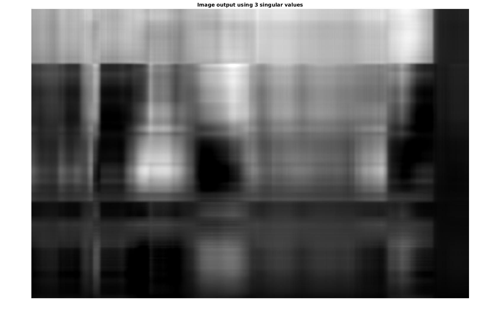
Here is the rendering of the partial sum of the three summands. Hard to know what this image is.

Figure 3.6.14. Image output using first three summands of SVD

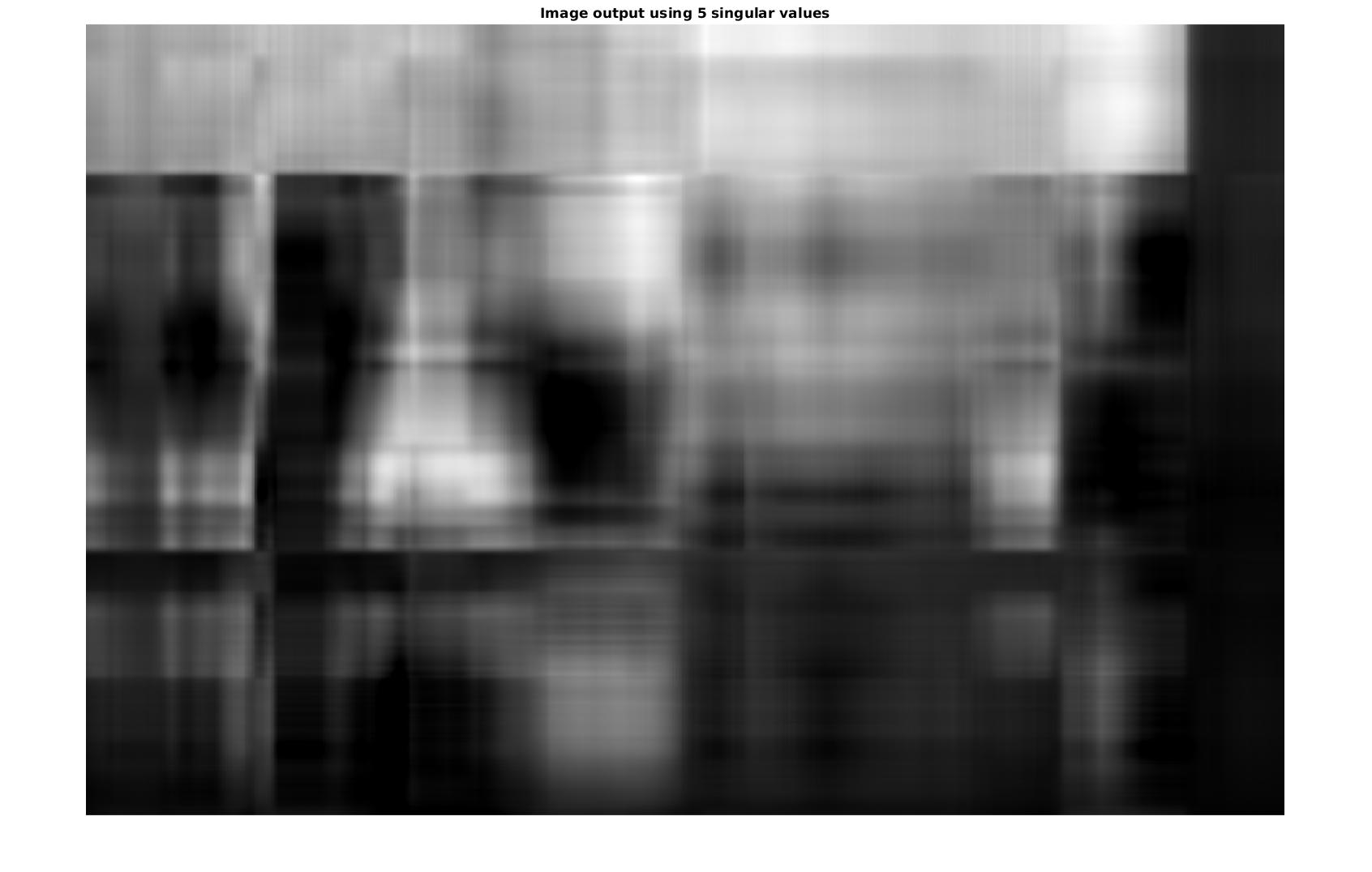
Even with the partial sum of 5 summands, interpreting the image is problematic, but remember it takes 1463 to render all the detail. But also, once you know what the image is, you will come back to this rendering and already see essential features.

Figure 3.6.15. Image output using first five summands of SVD

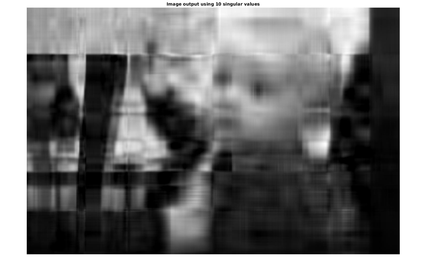
Below are the renderings of partial sums with 10, 15, 25, 50, 100, 200, 500, 1000, and all 1463 summands. Look at successive images to see how (and at what stage) the finer detail is layered in. Surely with only 10 summands rendered, there can be no question of what the image is.

Figure 3.6.16. Image output using first 10 summands of SVD

Figure 3.6.17. Image output using first 15 summands of SVD

Figure 3.6.18. Image output using first 25 summands of SVD

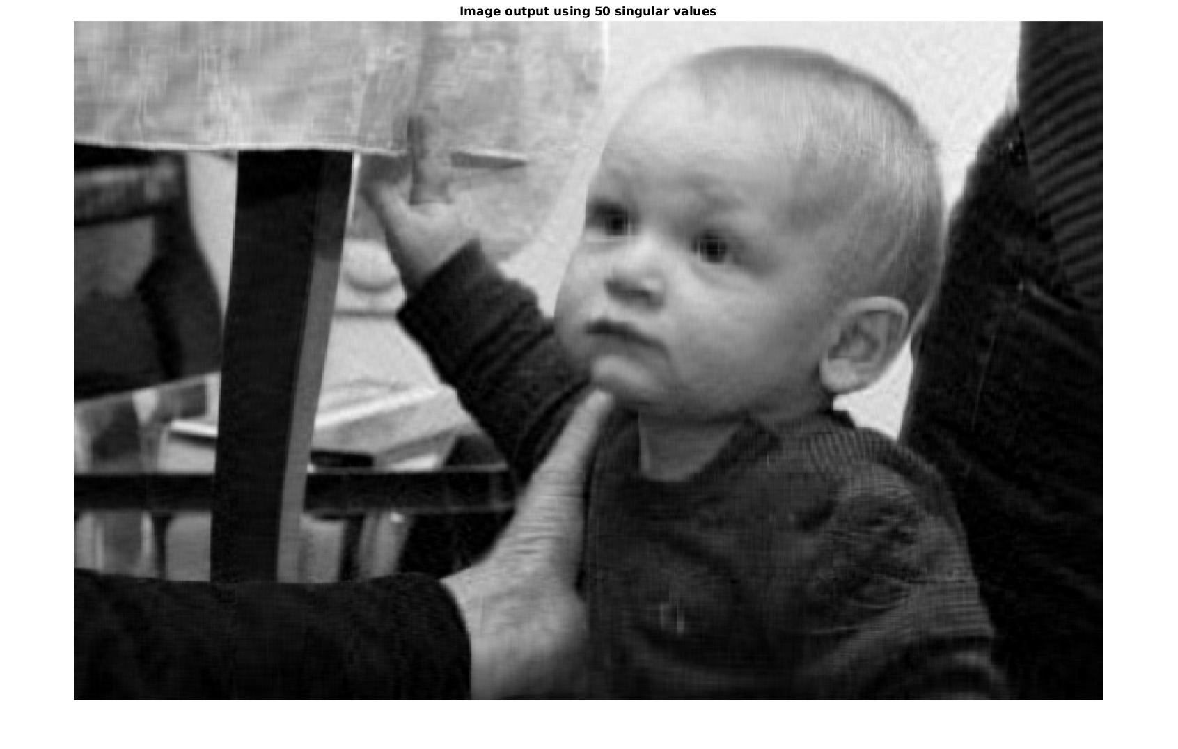
Figure 3.6.19. Image output using first 50 summands of SVD

Figure 3.6.20. Image output using first 100 summands of SVD

Figure 3.6.21. Image output using first 200 summands of SVD

Figure 3.6.22. Image output using first 500 summands of SVD

Figure 3.6.23. Image output using first 1000 summands of SVD

Figure 3.6.24. Original image (all 1463 summands)

Subsection 3.6.8 Some parting observations on the SVD

Back in Theorem 3.2.17 and Corollary 3.2.18 we defined the so-called four fundamental subspaces. Let us see how they are connected via the singular value decomposition of a matrix.

We started with an \(m\times n\) matrix \(A\) having rank \(r\text{,}\) and an SVD of the form \(A=U\Sigma V^*:\)

\begin{equation} [\underbrace{ u_1\ \cdots u_r}_{\col A}\ \underbrace{ u_{r+1} \cdots u_m}_{\ker A^*}] \ba{c|r} \begin{array}{rrr}\sigma_1\amp\amp0\\\amp\ddots\\0\amp\amp\sigma_r\end{array} \amp\0\\\hline\0\amp\0\ea \ba{r} v_1^*\\\vdots\\ v_r^*\\ v_{r+1}^*\\\vdots\\ v_n^*\ea \begin{array}{l} \left.\rule{0pt}{25pt}\right\}\col A^*\\ \left.\rule{0pt}{25pt}\right\}\ker A \end{array}\tag{3.6.2} \end{equation}

We have the orthonormal basis \(\{u_1, \dots, u_m\}\)for \(\C^m\) of which \(\{u_1, \dots, u_r\}\) is an orthonormal basis for \(\col A\text{,}\) the column space of \(A.\) So that means that \(\{u_{r+1},\dots, u_m\}\) is an orthogonal subset of \((\col A)^\perp = \ker A^*\) by Theorem 3.2.17.

By Corollary 3.2.11, we know that \(\C^m = \col A \boxplus (\col A)^\perp,\) so

\begin{equation*} m = \dim \C^m = \dim \col A + \dim (\col A)^\perp, \end{equation*}

so \(\dim (\col A)^\perp = m -r,\) and it follows that \(\{u_{r+1},\dots, u_m\}\) is an orthonormal basis for \((\col A)^\perp = \ker A^*\text{.}\)

Turning to the right side of the SVD, we know that

\begin{equation*} \|Av_i\| = \sigma_i \text{ for } i = 1, \dots, n, \end{equation*}

and by the choice of \(r\text{,}\) we know that

\begin{equation*} Av_{r+1} = \cdots = Av_n = 0. \end{equation*}

Since the \(\rank A = r\text{,}\) the \(\nullity A = n-r\) which means that \(\{v_{r+1},\dots, v_n\}\) is an orthonormal basis for \(\ker A.\)

Finally it follows that \(\{v_1, \dots, v_r\}\) is an orthonormal basis for \((\ker A)^\perp = \col A^*\text{.}\) Note that when \(A\) is a real matrix, \(\col A^* = \col A^T = \row A.\)

In display (3.6.2), we have seen a certain symmetry between the kernels and images of \(A\) and \(A^*,\) and in part we saw that above in Subsection 3.6.4 where we used the SVD for \(A^*\) to obtain one for \(A.\) We connect the dots a bit more with the following observations.

In constructing an SVD for \(A = U\Sigma V^*\text{,}\) we had an orthonormal basis \(\{v_1, \dots, v_n\}\) which were eigenvectors for \(A^*A\) with eigenvalues \(\lambda_i = \sigma_i^2.\) Noting that \(\|Av_i\| = \sigma_i,\) we set \(\ds u_i = \frac{1}{\sigma_i} Av_i\) for \(i=1,\dots, r\text{,}\) observed it was an orthormal set and extended in to an orthonormal basis \(\{u_1, \dots, u_m\} \) for \(\C^m.\)

From the definiton, \(u_i = \frac{1}{\sigma_i} Av_i\) we see that \(Av_i = \sigma_i u_i.\) What do you think \(A^*u_i\) should equal?

We compute

\begin{equation*} A^*u_i = \frac{1}{\sigma_i}A^*(Av_i) = \frac{1}{\sigma_i}(A^*A)v_i= \frac{1}{\sigma_i}\lambda_i v_i = \sigma_i v_i. \end{equation*}

Thus we have the wonderfully symmetric relation:

\begin{equation*} Av_i = \sigma_i u_i \text{ and } A^* u_i = \sigma_i v_i \text{ for } i=1, \dots, r. \end{equation*}

Typically in a given singular value decompostion, \(A=U\Sigma V^*\text{,}\) the columns of \(U\) are called the left singular vectors of \(A,\) while the columns of \(V\) are called the right singular vectors.

Prev Top Next