
Section 1.11 The precise definition of the limit
Now that we have some intuition about limits and tools to evaluate them, we turn to refining our rough definition to make it precise. Objectives
Let's first remind ourselves of our rough definition of the limit.
Definition 1.11.1.
Let \(f(x)\) be a function defined at all values in an open interval containing \(a\text{,}\) with the possible exception of a itself, and let \(L\) be a real number. If all values of the function \(f(x)\) approach the real number \(L\) as the values of \(x\) (that are not equal to \(a\)) approach the number \(a\text{,}\) then we say that the limit of \(f(x)\) as \(x\) approaches a is \(L\text{.}\) (More succinct, as \(x\) gets closer to \(a\text{,}\) \(f(x)\) gets closer and stays close to \(L\text{.}\)) Symbolically, we express this idea as
But this isn't quite enough - we also have the idea that "as \(x\) gets closer to \(a\text{,}\) \(f(x)\) gets closer and stays close to \(L\text{.}\)" This is a little harder to get at, we want to quantify the idea that as \(|x-a|\) gets smaller, so does \(|f(x)-L|\) but they might be getting smaller at different rates - e.g. when \(|x-a|=0.001\text{,}\) we could have \(|f(x)-L|=0.451\text{.}\) How do we get at this? The key idea is a little subtle. We want to ensure that \(f(x)\) gets closer and closer to \(L\text{,}\) so we can think of this as a game of sorts - if you give me a really small number, which we will call \(\epsilon\text{,}\) I need to be able to find a perhaps different number, which we call \(\delta\text{,}\) with the property that for all values of \(x\) where \(0 < |x-a|<\delta\text{,}\) we have that \(|f(x)-L|<\epsilon\text{.}\)
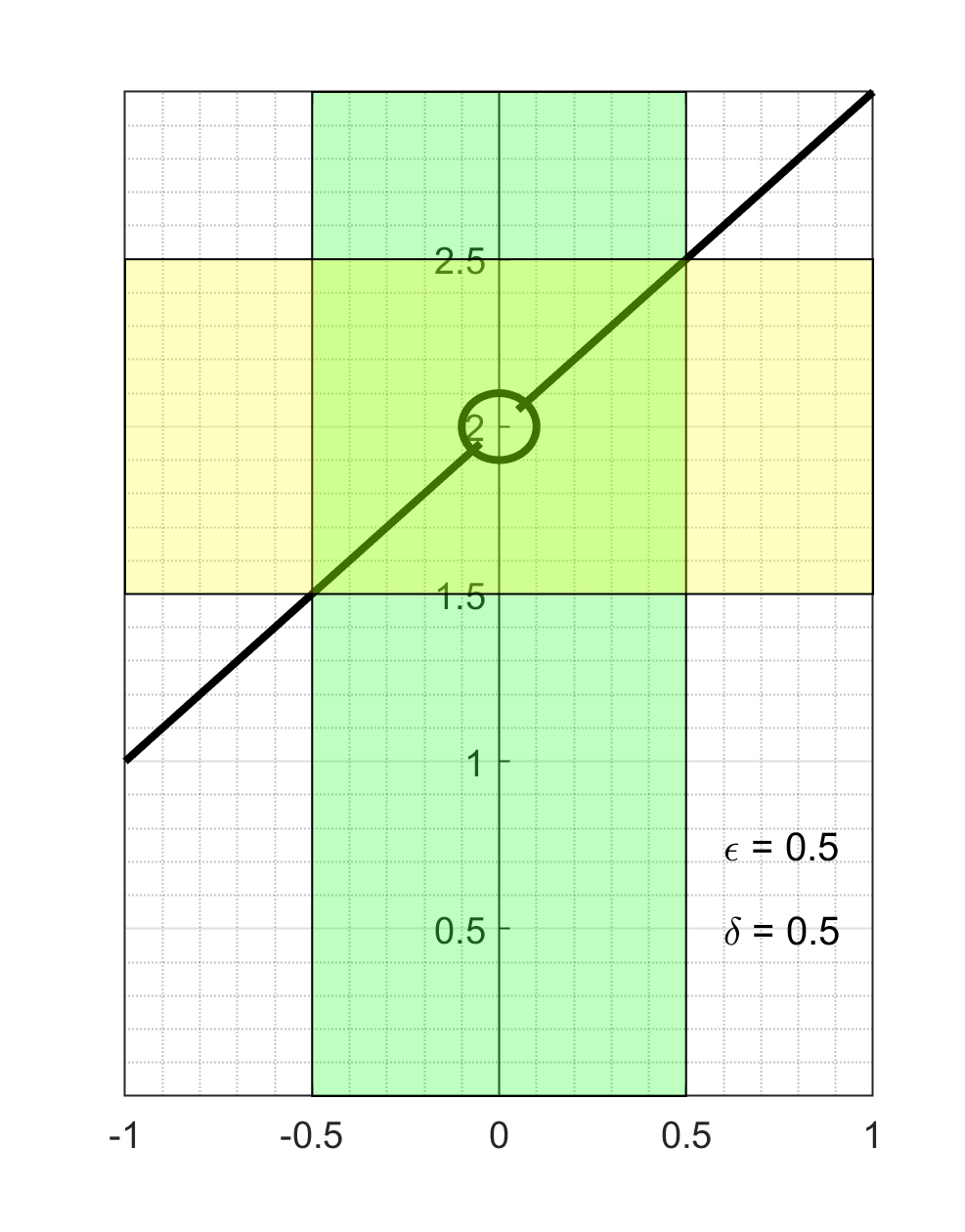
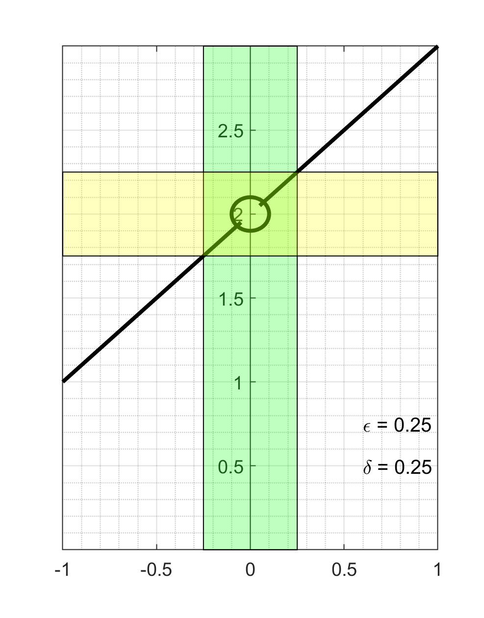
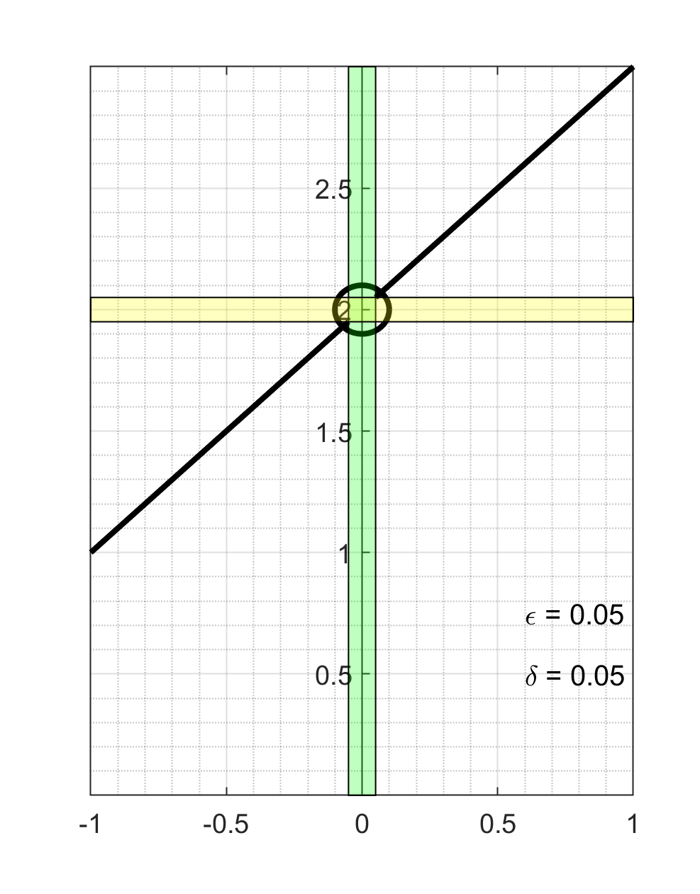
Figure 1.11.2 shows an example of several different \(\epsilon\) and \(\delta\) pairs. This example comes from a calculation we did in a previous video when we looked for the slope of the tangent line to \(f(x)=x^2\) at \(x=1\) by taking the limit of slopes of secant lines. The limit we arrived at was
Away from zero, this rational function simplifies to the linear function \(2+h\text{,}\) which gives us the black line in each of the panels. The circle highlights the missing point where the function is not defined. The green rectangle shows the band of width \(2 \delta\) centered at zero and the yellow rectangle shows the band of width \(2 \epsilon\) centered on the possible limiting value. We can see that at least for these three \(\epsilon\)'s we can find \(\delta\)'s so that if \(0 < |x-a|<\delta\text{,}\) then \(|f(x)-L|<\epsilon\text{.}\)
The key to the definition of a limit is that this has to work no matter what \(\epsilon\) is, we need to be able to find a \(\delta\text{.}\)
Definition 1.11.3.
Let \(f(x)\) be defined for all \(x \neq a\) over an open interval containing \(a\text{.}\) Let \(L\) be a real number. Then
We start with the last part, \(|f(h)-L|<\epsilon\text{,}\) and thinking of \(\epsilon\) as a small fixed number bigger than zero. Plugging in our function definition and using the graphs get the estimate of \(2\) for the limit, we have \(\left | \frac{2h+h^2}{h}-2\right | < \epsilon\text{.}\) Since we are looking at values of \(h\) that are close to but not equal to zero, we can cancel a factor of \(h\) from the top and bottom of the fraction:
which simplifies to
Now we can compare this to the first part of the if-then statement in the defintion:
Since \(a=0\text{,}\) this simplifies to \(|h| < \delta\text{.}\) The goal now is to use compare these two inequalities to write \(\delta\) as a function of \(\epsilon\text{.}\) In other words, we want a rule that takes an \(\epsilon\) as an input and outputs a \(\delta\) for which the if-then statement is true. This case is pretty simple - we can pick \(\delta=\epsilon\) as the two inequalities have the same form.
This gives you a first look at the formal definition of the limit and an example of using it in practice. In our next video, we will do several more examples to further illustrate the definition.