
Section 1.8 The Squeeze Theorem
In our last two videos, we learned about a few different tools to help us evaluate limits. Next, we turn to one more technique, the Squeeze Theorem. Objectives
The squeeze theorem provides us with a new tool that can get at some of these problems. The basic idea is to use limits you already know how to compute to give us information about the limit we don't know. This idea has a direct line to Archimedes method of exhaustion where he "squeezed" the value of \(\pi\) between perimeters of polygon that he could calculate. We've also seen a version of this idea in our last video when we took advantage of cancellation in some examples to build a function that had the same limit as our problem, but that we could easily take the limit of. When we try to take the limit
we recognize that
at all values of \(x\) except possibly at \(x=2\text{.}\) So the two functions have the same limit there, and we can use limit laws to evaluate
The squeeze theorem combines this idea with approximation. Suppose we have a limit we want to find,
We want to find two functions for which we can compute the limit, call them \(f(x)\) and \(h(x)\) that bracket our function. In other words we want
for all values nearby to zero. If \(\lim_{x \rightarrow 0}f(x)=L\) and \(\lim_{x \rightarrow 0} h(x)=M\) and we take the limit of all the parts of this set of inequalities, then we get
or
Now this tells us something about the limit - it is between L and M - but still doesn't give us the complete answer. The trick now is to find an \(f(x)\) and \(g(x)\) so that \(L=M\) - then the computation above would imply that \(\lim_{x \rightarrow 0}x \cos(x)=L\text{.}\)
But how in the world can we find these functions? Sadly, there is no formula or recipe for doing this - we need to think about \(x\) and \(\cos(x)\) and see what we can figure out. Let's start by looking at the graph of \(\cos(x)\) over one of its periods in Figure 1.8.1. 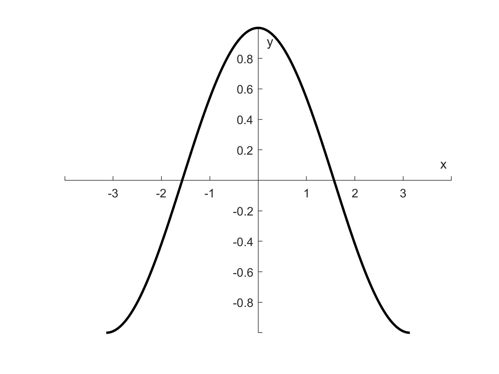
and for negative values of x, we have
This makes this a little complicated - to help us we will introduce a new notion, the one sided limit. When we made our somewhat informal definition of the limit, we thought about what value the function tended to as we approached the \(x\) value from both sides. A one-sided limit has a similar definition but we only consider values from the right or left of the limiting \(x\) value. We use a modified notation as well:
when we only look at values to the right of \(a\) and
when we only consider values to the left. The two-sided limit exists if both one-sided limits exist and are equal to the same value.
Let's apply this idea here to try to find \(\lim_{x \rightarrow 0}x \cos(x)\text{.}\) First, we'll look at values to the right of zero - positive values of \(x\text{.}\) Taking the one-sided limit of the series of inequalities, we have
Now both the functions \(f(x)=-x\) and \(h(x)=x\) are polynomials so we can find their limits by evaluation:
Since these are equal, we conclude
If we only consider values to the left- negative x values- we have a similar computation:
and we conclude that
as well. Taken together, this tells us that the limit of \(x \cos(x)\) as \(x\) approaches zero is zero.
This is the essence of the Squeeze Theorem: Let \(f(x),g(x)\text{,}\) and \(h(x)\) be defined for all \(x \neq a\) over an open interval containing \(a\text{.}\) If for all \(x \neq a\) in an open interval containing \(a\) and where \(L\) is a real number, then \(\lim_{x \rightarrow a} f(x)=L\text{.}\)
Theorem 1.8.2. The Squeeze Theorem.
Just like in our example, the function \(g(x)\) is squeezed between two functions and because those function have the same limit at \(a, g(x)\) has that limit too.