
Section 1.2 Classes of functions
In our last video, we reviewed the notion of a function and some of their properties, like the domain and range. Next, we turn to reviewing a few of the most useful classes of functions. Objectives
The highest power of \(x\) of a polynomial is called the degree, and we most often look at polynomials of lower degree like lines,
quadratics,
and cubics,
Trigonometric functions form our second class of functions. These include \(\sin(x), \cos(x), \tan(x),\sec(x),\csc(x),\cot(x)\text{.}\) The sine and cosine functions are the most basic trigonometric functions - all of the others can be constructed from them. But how are they defined? Sine and cosine arise when we think about circles. Let's look at a circle of radius one in Figure 1.2.1, and a point on that circle shown in green. That point can be identified by measuring the angle,\(\theta\text{,}\) from the horizontal axis. We define \(\sin(\theta)\) and \(\cos(\theta)\) as the vertical and horizontal coordinates of the green point respectively. Because these functions are so tightly linked to the circle, there are lots of relations between them. The simplest and most useful identity comes from the algebraic definition of the circle,
Since every point on the circle satisfies this equation, and \((\sin(\theta),\cos(\theta))\) defines a point on the circle for every \(\theta\) we have that
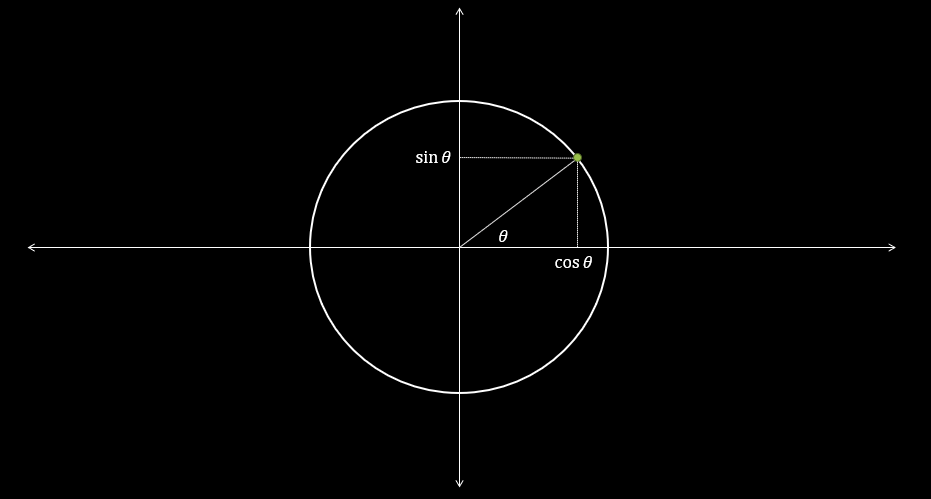
We can't write down a simple rule for sine or cosine, we can get a sense of what their graph looks like by think about their defintion using the circle. If we start at the point \((1,0)\) which corresponds to \(\theta = 0\text{,}\) this gives us that \(\sin(0)=0\text{.}\) If we increase \(\theta\) the point moves around the circle and if we keep track of the vertical coordinate, it will plot the points on the graph of the sine curve. Figure 1.2.2 demonstrates this graphically.
While there are lots of other useful identities, we won't go through them here. Instead, we will review them as they arise in our other investigations. But, it is important to point out how the other trigonometric functions are related to sine and cosine, which is summarize in Table 1.2.3.
| \(\tan(\theta)=\frac{\sin(\theta)}{\cos(\theta)}\) | \(\cot(\theta)=\frac{\cos(\theta)}{\sin(\theta)}\) | ||
| \(\sec(\theta)=\frac{1}{\cos(\theta)}\) | \(\csc(\theta)=\frac{1}{\sin(\theta)}\) |
Our third class of functions includes the exponential and logarithmic functions. Exponential functions are a good example of a function that serves as a model for a process. In this case, the process is a particular common type of growth. Whenever you have something - a population, a bank account, etc. - that grows propotionally to its current size the exponential function is a good model.
Let's think about the example of a population of organisms. Over time, the organisms reproduce. While different organisms reproduce in different ways and at different rates, one thing they all have in common is that only living organisms have the potential to reproduce. So, we can conclude that the amount a population will change over a given time period is proportional to the size of the population itself. This sweeps a lot under the rug - all those details about reproduction - and is a little bit wrong as we can easily end up in a situation where the population growth would include fractions of organisms. But, it turns out to be a really useful simplified model.
If we think about how this plays out mathematically, we can start with an initial population, \(P(0)\text{,}\) and a rate of growth, \(r\text{.}\) After one unit of time, our population is \(P(1)=P(0)+rP(0)=P(0)(1+r)\) and after two units of time the population is \(P(2)=P(1)+rP(1)=P(1)(1+r)=P(0)(1+r)^2\text{.}\) If we keep writing down the population at further time points we start to see a pattern
This is an example of an exponential function. The general form of these functions is
where \(c\) and \(b\) are constants and \(x\) is the variable. We call \(b\) the base of the exponential function.
To introduce the logarithm, we need to talk first about inverse functions. If we return to our metaphor of a function as a machine that takes input and produces outputs, the inverse of the function runs the machine backwards, transforming the outputs into the inputs they came from. Consequently, if our functions turns \(x\) into \(f(x)\) then the inverse should turn \(f(x)\) back in to \(x\text{.}\) If we denote the inverse of \(f\) by \(f^{-1}\text{,}\) then it is characterized by the either
or
Generally, inverses are hard to compute but we can often use them to define new functions whose properties we can understand even if we can't exactly write down a rule for them. This is how we define the logarithm. If our exponential function is given by \(b^x\) then we denote its inverse by \(log_b\) so that \(log_b(b^x)=x.\) Figure 1.2.4 shows a few different exponential functions and their inverses.